Alignments and WER

In this guide we first provide quick start examples. Then we describe in details the processing pipeline, from tokenizing to dataset summarizing. Finally, we describe our alignment algorithm from the mathematical point of view.

Quick start

Installation

For current section, installing via pip install asr_eval will be enough. See Installation for more details.

What is Word Error Rate?

Word Error Rate (WER) is a ratio of wrongly transcribed words, including missing or extra words.

\[WER = \frac{\text{Insertions} + \text{Deletions} + \text{Replacements}}{\text{Number of words in the annotation}}\]

To calculate it, we take the predicted transcription and the annotation, and split both of them into words. Then we perform a sequence alignment to match both word sequences. This is best shown with an example below.

Aligning against multi-reference transcription

asr_eval supports multi-reference and wildcard syntax for annotation. Imagine a child interrupts a blogger with a babble. We have difficulty recognizing this speech, and the transcription model might even skip it altogether as a background speech/vocalizations, which is not a mistake. Therefore, we annotate it as <*>:

true = '{Now...} now take a plank {1|one} {m|meter|metre} long. <*> Well!'
pred = 'No! Take blank one meter long, Daddy, daddy. Well!'

Let’s tokenize it with the DEFAULT_PARSER and align with the Alignment class:

from asr_eval.align.alignment import Alignment
from asr_eval.align.parsing import DEFAULT_PARSER

true_parsed = DEFAULT_PARSER.parse_transcription(true)
pred_parsed = DEFAULT_PARSER.parse_single_variant_transcription(pred)

alignment = Alignment(true_parsed, pred_parsed)
metric, errors = alignment.error_listing(max_consecutive_insertions=4)
print('WER:', metric.word_error_rate(clip=True))

WER: 0.375

Let’s see how it was aligned:

from IPython.display import display, HTML  # doctest: +SKIP
display(HTML(alignment.render_as_text(color_mode='html')))  # doctest: +SKIP

true | {Now...} now take a plank {1|one} {m|meter|metre} long <*> Well
pred | No Take blank one meter long Daddy daddy Well

We see that <*> was aligned with “Daddy, daddy”, “a” was skipped in the transcription and thus considered a mistake, and the repetition “Now…” is marked as optional: skipping it is not a mistake. Overall, we found 3 mistakes, and the ground truth length is 8 words (in each multi-reference blocks we consired the shortest option), thus WER = 3/8 = 0.375.

We can also visualize how the texts were split into words. In general, each multi-reference option can contain more than one word.

from IPython.display import display, HTML
display(HTML(true_parsed.colorize(color_mode='html')))
display(HTML(pred_parsed.colorize(color_mode='html')))

{Now...} now take a plank {1|one} {m|meter|metre} long. <*> Well!
No! Take blank one meter long, Daddy, daddy. Well!

The resulting Metrics object contains more information:

print(metric)

Metrics(true_len=8, n_replacements=2, n_insertions=0, n_deletions=1)

Let’s enumerate all the errors:

for error_pos in errors.values():
    print(f'Predicted "{error_pos.pred_text}" instead of "{error_pos.true_text}"')

Predicted "no" instead of "now"
Predicted "" instead of "a"
Predicted "blank" instead of "plank"

WER settings

In the example, we use max_consecutive_insertions=4 to treat more than 4 consecutive insertions as exactly 4 (relaxed insertion penalty) and clip=True to clip WER between 0 and 1. Remove this paramters if this is not needed in your case, to get the standard WER.

Performance note

Currently, our alignment algorithm can be slow for long recordings (10+ minutes of speech). While our algorithm is O(n^2), same as the Needleman–Wunsch algorithm, our implementation (asr_eval.align.solvers.dynprog.solve_optimal_alignment()) is pure Python-based and may be inefficient. We plan to speed up the code soon.

Multiple alignment

Let we have several different transciptions. We align them all against the annotation and display in one block:

from asr_eval.align.alignment import Alignment
from asr_eval.align.parsing import DEFAULT_PARSER
from asr_eval.align.alignment import MultipleAlignment

true = '{Now...} now take a plank {1|one} {m|meter|metre} long. <*> Well!'
preds = {
    'model1': 'No, no! Take a blank one meter long, Daddy, daddy. Well!',
    'model2': 'NOW TAKE A PLANK 1 METRE LONG DADDY DAAA WELL',
    'model3': 'no now I\'ll take a blank 1 M long',
}
true_parsed = DEFAULT_PARSER.parse_transcription(true)
alignments = {
    name: Alignment(true_parsed,
        DEFAULT_PARSER.parse_single_variant_transcription(pred))
    for name, pred in preds.items()
}
ma = MultipleAlignment(true_parsed, alignments)

from IPython.display import display, HTML
display(HTML(ma.render_as_text(color_mode='html')))

true | {Now...} now take a plank {1|one} {m|meter|metre} long <*> Well
model1 | No no Take a blank one meter long Daddy daddy Well
model2 | NOW TAKE A PLANK 1 METRE LONG DADDY DAAA WELL
model3 | no now I ll take a blank 1 M long

Character error rate

You can find the example of defining a custom parser that enables CER calculation instead of WER in this section.

Summarizing a dataset

Installation

For this section, we need a support for ASR models and datasets. Please install the required packages: pip install asr_eval[datasets,models_stable].

Let’s retrieve a Russian dataset Podlodka-speech. It is annotated with a normal single-reference annotation.

from asr_eval.bench.datasets import get_dataset
from asr_eval.models.whisper_wrapper import WhisperLongformWrapper
from tqdm.auto import tqdm

dataset = get_dataset('podlodka')
print(dataset)

Dataset({
    features: ['audio', 'transcription', 'episode', 'title', 'sample_id'],
    num_rows: 20
})

We now run the model for each sample and align the results.

from dataclasses import dataclass, field
from asr_eval.align.alignment import ErrorListingElement, Alignment
from asr_eval.align.metrics import Metrics
from asr_eval.align.parsing import DEFAULT_PARSER
from asr_eval.models.base.interfaces import Transcriber
from datasets import Dataset

@dataclass
class RunResults:
    alignments: list[Alignment] = field(default_factory=list)
    metrics: list[Metrics] = field(default_factory=list)
    errors: list[list[ErrorListingElement]] = field(default_factory=list)

def run_on_dataset(dataset: Dataset, model: Transcriber) -> RunResults:
    results = RunResults()

    for sample in tqdm(dataset):
        pred = model.transcribe(sample['audio']['array'])

        pred_parsed = DEFAULT_PARSER.parse_single_variant_transcription(pred)
        true_parsed = DEFAULT_PARSER.parse_transcription(sample['transcription'])
        alignment = Alignment(true_parsed, pred_parsed)
        metric, errors_for_sample = alignment.error_listing()

        results.alignments.append(alignment)
        results.metrics.append(metric)
        results.errors.append(list(errors_for_sample.values()))

    return results

model = WhisperLongformWrapper('openai/whisper-tiny')
whisper_tiny_results = run_on_dataset(dataset, model)

Now let’s calculate dataset WER and bootstrap intervals.

import numpy as np
from asr_eval.align.metrics import DatasetMetric

metrics = whisper_tiny_results.metrics

print(f'WER (macro-averaging): {np.mean([m.word_error_rate() for m in metrics]):.3f}')
print(f'WER (micro-averaging): {sum(metrics).word_error_rate():.3f}')

# use wer_averaging_mode='concat' (default) for micro-averaging
# and 'plain' for macro-averaging
dataset_metric = DatasetMetric.from_samples(metrics, wer_averaging_mode='concat')
wer_lower, wer_upper = dataset_metric.wer.quantiles((0.1, 0.9))
print(f'WER (micro-averaging) bootstrap interval: ({wer_lower:.3f}, {wer_upper:.3f})')

WER (macro-averaging): 0.363
WER (micro-averaging): 0.372
WER (micro-averaging) bootstrap interval: (0.338, 0.408)

Now let’s add another model and compare them on plots. By default plots use (0.1, 0.9) bootstrap quantiles for confidence intervals.

from asr_eval.align.metrics import DatasetMetric
from asr_eval.align.metrics import plot_dataset_metric

model = WhisperLongformWrapper('openai/whisper-small')
whisper_small_results = run_on_dataset(dataset, model)

plot_dataset_metric({
    'whisper-small': DatasetMetric.from_samples(whisper_small_results.metrics),
    'whisper-tiny': DatasetMetric.from_samples(whisper_tiny_results.metrics),
}, what='wer')

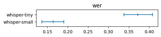
We discuss model comparison in more details in the next sections.

Fine-grained analysis for a dataset

Let’s now analyze which words are most frequently transcribed wrongly.

all_errors = sum(whisper_tiny_results.errors, [])

from collections import defaultdict
from collections import Counter

errs_grouped: dict[str, list[str]] = defaultdict(list)
for err in all_errors:
    if err.true_text and len(err.true_text) > 3:  # skip insertions and short words
        errs_grouped[err.true_text].append(err.pred_text)

# sort by number of errors
errs_grouped_sorted = sorted(errs_grouped.items(), key=lambda x: -len(x[1]))

for true_text, pred_texts in errs_grouped_sorted[:10]:
    deleted = [p for p in pred_texts if not p]
    replaced = [p for p in pred_texts if p]
    most_common_replaced = [w for w, _i in Counter(replaced).most_common(3)]
    print(
        f'"{true_text}" was replaced {len(replaced)} times: {most_common_replaced}'
    )

"нейронные" was replaced 4 times: ['неронной', 'неронные', 'нейроносите']
"наше" was replaced 3 times: ['наши']
"кандидатов" was replaced 3 times: ['полкандитатов', 'кандитатов']
"этот" was replaced 2 times: ['это']
"нету" was replaced 2 times: ['нет']
"тимлидом" was replaced 2 times: ['темлидом']
"пайплайн" was replaced 2 times: ['pipeline', 'поеплайн']
"всего" was replaced 2 times: ['его', 'все']
"задаче" was replaced 2 times: ['задачи']
"данные" was replaced 2 times: ['данный', 'самеданной']

This quickstart section showcased the possibilities of the align module. The next section describes in more details all stages of the evaluation pipeline and discusses the challenges.

Detailed processing pipeline

This section is in progress.

We plan to describe the following in more detail:

1. Tokenization and parsing. When labeling a dataset, the annotator should be aware of the tokenization scheme. For example, if 3/4$ is tokenized as a single word, then 3/4$ and 3 / 4 $ (with spaces) are different options, and both should be included in a multi-reference block. If we annotate only “3/4$”, then a prediction “3 / 4 $” will be considered 4 errors. On the other side, if we split by space, we need to enumerate a lot of options for “3/4$!”. The current regexp treats as word either a continuous sequence of word characters only (\w+), or a continuous sequence of [^\w\s{PUNCT}]+ - that is, a sequence of any characters excluding letter, space or punctuation ones. Thus, in the above example, there is no punctuation symbols, and the result will be the same [“3”, “/”, “4”, “$”] for both “3/4$” and “3 / 4 $”. However, there are still limitations with our method: for example, if “16-й” is a correct transcription, then “16 й” will always be considered correct. We will also discuss a well-known nltk.wordpunct_tokenize algorithm that searches for either \w+ or [^\w\s]+ matches. It does not allow to separate symbols such as dollar sign from punctuation: “$!” will be considered a single token. Finally, we will descibe our Transcription format which keep the positions of each tokenized word in the original text.

from asr_eval.align.parsing import DEFAULT_PARSER

text = (
    '(7-8 мая) в Пуэрто-Рико прошёл {шестнадцатый|16-й|16}'
    ' этап "Формулы-1" с фондом 100,000$!'
)

transcription = DEFAULT_PARSER.parse_transcription(text)

from IPython.display import display, HTML
display(HTML(transcription.colorize(color_mode='html')))  # doctest: +SKIP

(7-8 мая) в Пуэрто-Рико прошёл {шестнадцатый|16-й|16} этап "Формулы-1" с фондом 100,000$!

2. Alignment and slots. We will describe how the our Alignment class constructor calls asr_eval.align.solvers.dynprog.solve_optimal_alignment() (for which we also have a legacy recursive implementation asr_eval.align.solvers.recursive.solve_optimal_alignment()), and processes the results. We will describe the internal concept of “slots”. In short, each slot represents a specific position in the ground truth: before, at or after a word in the ground truth. However, things become more complicated for multi-reference transcription where we have inner and outer slots.

3. Multi-reference WER. For multi-reference annotations, defining WER is not straightforward. Selecting a specific variant in a multi-reference block also affects the reference length. Let we compare the prediction “B” against the reference “{A | B B B}”. If we select option “A”, we get edit distance 1 and WER = 1. If we select option “B B B”, we get higher edit distance 2 but lower WER = 2/3. Our alignment algorithm minimizes edit distance, as usual, but in rare cases this may not minimize WER in multi-reference annotations. This is not a big problem, though, because in WER metric the denominator plays the same role as sample weights. If we always use 1 as the denominator, this will be a sum of edit distances for all samples, that is similar to calculating WER on concatenation of samples, that is also a valid method. So, choosing a correct denominator is not crucial.

3. Multiple alignment. We will discuss multiple alignments. Note that we do not align multiple predictions against each other, but align the all against the ground truth (or the baseline prediction for unlabeled data). The MultipleAlignment class forms a table, where predictions are rows, and columns represent outer slots in the ground truth. In the rendering stage, we add the required count of spaces to make all cells in each column equally wide. Then we add ANSI color codes or HTML tags to mark errors.

4. Dataset averaging. Our experimental framework, described in Evaluation and dashboard, saves inference results incrementally, sample by sample. This is convinient in many cases, but complicates model comparision. We fisrt need to extract a set of samples for which all models generated predictions, and average by this set. We will discuss averaging modes (such as micro- and macro-averging) and confidence intervals. Interestingly, the difference between models can be statistically significant even if their confidence intervals overlap, what we will describe with examples.

Alignment algorithm

Our algorithm is a generalization of the Needleman–Wunsch algorithm to support multi-choice blocks and wildcard blocks (matching any sequence, possibly empty) for both sequences.

Flat view. We start by converting a multivariant annotation into a “flat view”. Our example contains 9 tokens (words) in total, including those inside and outside multivariant blocks. We arrange them into a list, prepend <start> and append <end> position. Then we define transitions between them, according to the multivariant structure. In our example, from the “<start>” word we can transit to “uh” or to “please” (skipping the {uh} optional block). The transitions are denoted as arrows on the vertical axis (for truth) and on the horizontal axis (for prediction).

Matrix position. It’s clear that a position in a resulting matrix means some pair of locations. More precisely, the matrix position “at token A in the annotation and token B in the prediction” means that these tokens were the last tokens we visited, that is, we are immediately after these tokens.

Matrix transition (step). A “step” is a transition between matrix positions. There are 3 types of transitions:

1. Vertical: transition over the annotation only. This means a “deletion” in terms of sequence alignment, because we go to the next token at the annotation while staying on the same position at the prediction.

2. Horizontal: transition over the prediction only. Similarly, this means an “insertion”.

3. Diagonal: transition over both the prediction and the annotation. This means either “correct” or “replacement”, depending on whether the tokens match or not.

Step score. Each step is associated with a score 0 or 1, depending on how much did the total number of errors increase after the step. A diagonal step may have a score 0 or 1, depending on whether the tokens match or not. The horizontal step is always 1, except cases where the current annotation token is wildcard - the score is 0 in this case, because we can step over any count of prediction tokens being at wilcard annotation token without incrementing error counter. The same for vertical step (however, the wildcard tokens in the prediction normally should not occur).

That is, we can traverse the matrix from the left lower to the right upper corner, or vice versa, and thus build an alignment, resulting in a final score (number of word errors) where we finish traversing both sequences.

Position score and best path. We define the best path for position as the lowest score path from the end to the current position. This is the same as the best alignment between the remaining parts of both sequences (from the current position to the end). The position score is a score of its best path. Our final goal is to find the best path for the (<start>, <start>) matrix position - this will be the optiomal sequence alignment.

Final positions. To start with, we define as “final” all the annotation positions leading directly to the <end> position, and the same for the prediction positions. In our example, 1 prediction position and 3 annotation positions are final (green), and the corresponding steps to the <end> are shown in green. We define a “final matrix position” as a combination of final annotation position and final prediction position (green dots). Being in a final martrix position, we are after final tokens in both sequences, that is essentially at the end. So, best path are empty for the final matrix positions, and their scores are zero.

Now we are going to fill the matrix from the final positions to the (<start>, <start>) position.

Matrix filling. Consider some matrix position X with unknown score and best path. Let S be a set of all matrix positions where we can get to in one step from X. In our example, the position X=(“please”, “oh”) contains 5 positions in S(X): 2 for vertical steps, 2 for diagonal and 1 for horizontal. Let’s assume that we know a position score for all positions in S(X). For each Xs ∈ S(X), we can calculate step_score(X, Xs) + score(Xs), and take the argmin across S(X) to find the best source position X*. Thus, score(X) = step_score(X, X*) + score(X*), and the best path for X consists of one step to X* plus the best path for X*.

Using the described process, we fill the whole matrix, starting from the last row from right to left, then the next row, and so on. Alternatively, we can fill the matrix column-wise or even diagonal-wise (which is the best to parallelze computations). Finally, we got a score for the position (<start>, <start>), which is the total number of word errors. To restore the best path (the alignment), it’s enough to keep the source position for each matrix position, and restore the path iteratively.

Complexity. Let A be the total word count in the annotation, and B be the total word count in the prediction. Also, let S(X) be bounded above (which is always the case in real multi-reference annotations). The complexity is O(AB) for the matrix propagation, since the number of operations to fill a cell is bounded above. The complexity of restoring the best path is O(max(A, B)) that is negligible comparing to O(AB). Thus, the overall complexity is O(AB). Since transcriptions B usually have length similar to the annotation A, the complexity is quadratic, as in the Needleman–Wunsch algorithm.

Improved scoring. There may be many cases where the argmin of step_score(X, Xs) + score(Xs) contains more than one source positions. This reflects the fact that there may be many optimal alignments. Across them all, we want to select those in which:

1. The number of correct matches is the highest.

2. The mismatched words have the least number of discrepancies in symbols.

This is straightforward to implement. Initially, we have a single score:

n_errors = n_replacements + n_deletions + n_insertions

We replace n_errors with a tuple of three scores:

1. n_errors

2. The number of correct matches in the path

3. Sum character errors for all the transitions int the path

These tuples are compared lexicographically: to compare (A1, B1, C1) with (A2, B2, C2) we first compare A1 with A2, if equal we compare B1 and B2, and if equal we finally compare C1 and C2. This ensures that the resulting best path is still optimal in terms of n_errors.

One possible alternative is to align on a character level (calculating CER instead of WER). Our algorithm is applicable also for this case. Note that such an alignment will not always be optimal in WER sense. This is stll a valid alternative, however, CER have its own biases (for example, it underestimates errors in word endings, since it’s only one or two characters).

Previous

Installation

Next

Streaming evaluation