Evaluation and dashboard¶

This guide contains 4 parts:

Dashboard quickstart. A quickstart from a CSV file with transcriptions.
Framework overview. An overview of our ASR-specific experimental framework.
Framework recipes. Adding datasets, models, running inference and dashboard.
Datasets usage. More details about the datasets in asr_eval.

Dashboard quickstart¶

Installation

For this section, please install the following packages: pip install asr_eval[datasets,ru_norm,dash].

The asr_eval package provides a dashboard to compare multiple models on multiple datasets, customize WER calculations and compare normalization strategies. This section describes a standalone dashboard usage, where both annotations and predictions are provided as CSV files.

We will use the example files provided in the docs/examples folder in the repo:

predictions.csv contains predictions and inference timings for GigaAM-v3-RNNT, GigaAM-v2-CTC and Whisper-v3-large on the first 20 samples of the dataset multivariant_v2.
annotations.csv contains the ground truth transcriptions for this dataset. As we descibe a standalone usage, we exported them into a separate CSV file.

Run the dashboard as follows:

cd docs/examples  # the csv files directory
python -m asr_eval.bench.dashboard.run -s predictions.csv -a annotations.csv

After the script prints “Dash is running”, open the provided URL, by default http://localhost:8051.

Some useful command line options (see asr_eval.bench.dashboard.run docs for details):

Use --host 0.0.0.0 to be able to connect from other IPs.
Use -d dataset(s), -p pipeline(s) to load only the specified datasets/pipelines from the file.
Use -c ./dashboard_cache to cache the string alignments into the specified cache directory. Note that if you change the predictions or annotations file, the cache will no longer be valid and you need to delete it.
You can omit -a (--annotations) for datasets registered in asr_eval (see Datasets list). You can also register custom datasets (see below).

To prepare your own data instead of example predictions.csv and annotations.csv, use the same format. You also can omit the “elapsed_time” rows in the CSV.

The dashboard selectors¶

The dashboard provides the following settings which are applied on “Show data”:

⚙️ Dataset selector. Select one of the datasets found in the predictions file. When using custom tokenizers or normalizers, this will also show which tokenizer or normalizer is used.

⚙️ Pipelines selector. Select one or more speech recognition pipelines to compare. By default, the asterisk means to select all the pipelines found in the predictions file. You can use any wcmatch expression to filter pipelines. For example, type *whisper*|*giga*|!*vad to select any pipeline name that contains whsiper or giga, but does not end with vad. This is useful when you compare plenty of configurations.

⚙️ Max samples to show. Limit the count of rendered sample to icnrease performance.

☑️ Export audio. If checked, on “Show data” will show a button to play each sample as audio. Note that this will result in error if the dataset is not registered in asr_eval, but only annotations are provided (see below how to register custom datasets). The audio is exported into the tmp/dashboard_assets directory (can be overriden with –assets_dir). You also can run the dashboard with –export-audio to pre-export all audio samples for all datasets, otherwise they will be exported on “Show data” click that may increase waiting time.

☑️ Exclude samples with digits. Will omit all samples that contain digit symbols 0-9 either in the annotation or in one of the predictions, and also exclude them from averaged metric calculation. This may be useful to mitigate issues with normalization of numerals. However, this introduces a spurious dependency between the pipeline set and the sample set. Also, this is meaningless for datasets with multi-reference labeling, such as multivariant-v2.

☑️ WER Settings -> Count absorbed insertions. When not checked, modifies WER calculations so that cases such as “nothing” -> “no thing” are treated as one word error but not two errors. The effect is usually negligible. See error_listing() for details.

⚙️ WER Settings -> Max consecutive insertions. When checked, treats more than X insertions (4 by default) as exactly 4, to stabilize metric against oscillatory hallucinations. See error_listing() for details.

⚙️ WER Settings -> Averaging mode. If “concat” (default), uses micro-averaging across samples, if “plain” uses macro-averaging. See Summarizing a dataset for details.

The dashboard outputs¶

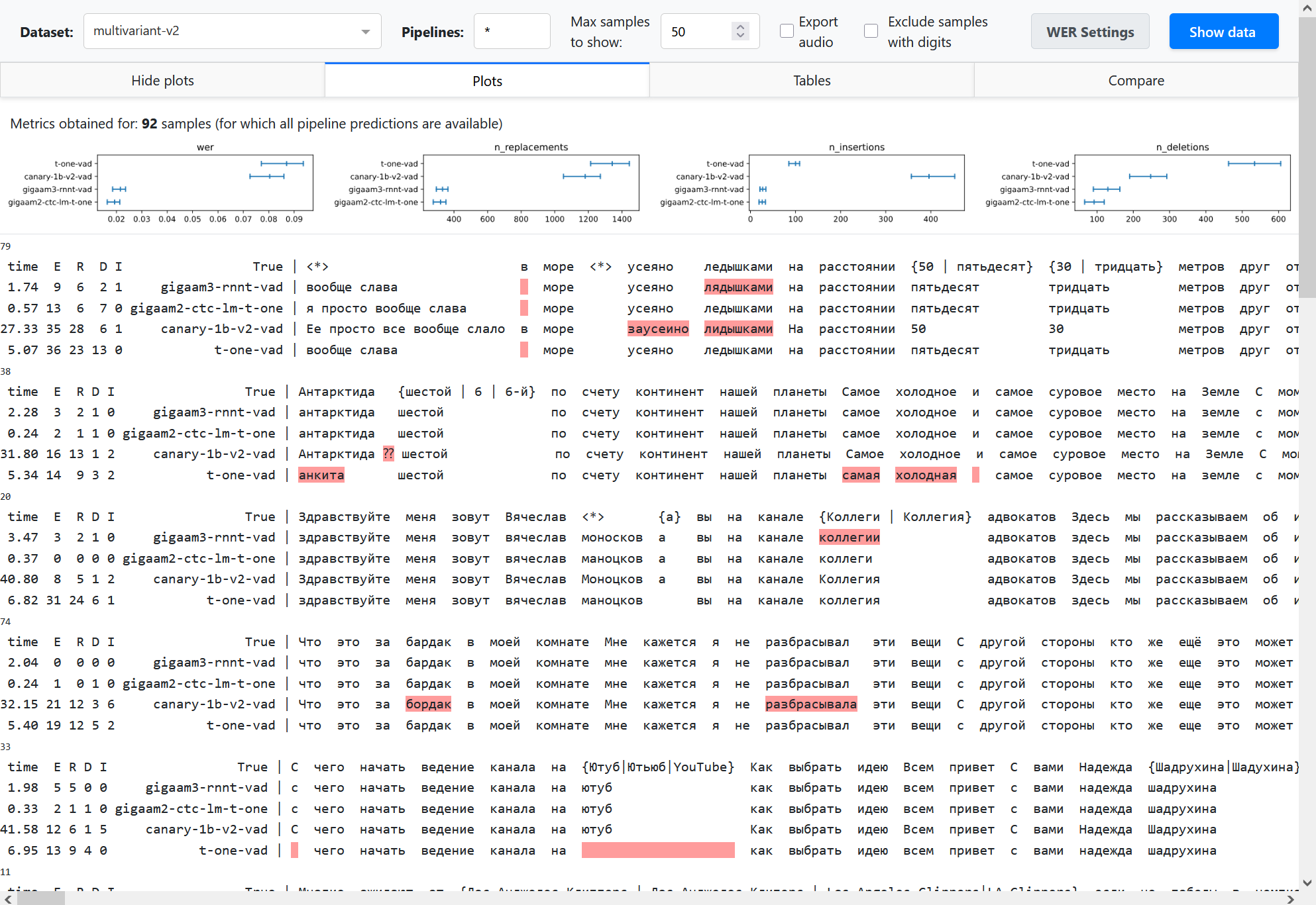
On Show data click the dashboard shows multiple alignments. Besides highlighting errors, it shows sample id (a number above alignment), inference time (if provided) and the numbers of replacements (R), deletions (D), insertions (I) and total errors (E).

In the Plots and Tables sections, it summarizes the metric over all the dataset to compare pipelines, using bootstrapping with quantiles 0.1 and 0.9 to determine confidence intervals (see Summarizing a dataset for details). The breakdown of the average WER into n_replacements, n_insertions and deletions plots can provide insights into model comparison.

Partial and incremental inference is enabled in our framweork for quick prototyping. However, this may lead to complexities in model comparison. We should compare pipelines on equal set of samples. To summarize metric, the dashboard uses only those samples for which all the provided pipelines have predictions. For example, if pipelines A and B have 100 predictions, and pipeline C have only a prediction for 10 samples, the metric averaging will be performed over 10 samples (that is stated explicitly above the plots). To avoid such a situation, it is also possible to reject pipelines with partial predictions using dataset specs in command line arguments.

In the Compare section, you can compare a pair of pipelines. Let’s call word occurence a specific occurrence of some word in the annotation of a specific example, and let’s call a word spelling simply a word as a sequence of letters that can occur multiple times. For example, a word “Alexa” may have 20 word occurences in the dataset. We compare the pipelines as follows.

We attribute each speech recognition error either to a word occurence in the annotation (replacement or deletion) or to nothing (insertion).
We find all word occurences in the annotation where both pipelines made an error. We count them as shared errors (blue bar on the plot). Note that shared errors counter may be slightly different for both pipelines, because some word occurence may be transcribed as 2 words and thus increment the WER error counter by 2.
We fint all insertions and count them as insertions (pink bar on the plot).
All other errors are considered unique - they are attrubited to word occurences where only one model did a mistake, and the other model transcribed correctly. These cases are the most interesting where we compare models. They form the rest of the bars on the plots. Some most common cases (grouped by word spellings) are shown explicitly, others are shown as other unique.

Notes

This example uses CSV files, which are human-readable, but inefficient at large scale and limiting in the types of data stored. Consider using database files, as suggested in the next sections.
If you just need to render multiple alignments for a single dataset, the dashboard may be an overhead. You can render each sample into HTML as described in Multiple alignment guide, and concatenate via <br> into a single .html file.

The files predictions.csv and annotations.csv can be reproduced by installing the requirements from the Framework recipes section and running the following commands:

python -m asr_eval.bench.run -s predictions.csv -d multivariant-v2:n=20 \
   -p whisper-large-v3 gigaam3-rnnt-vad gigaam2-ctc --keep text elapsed_time
python -m asr_eval.bench.datasets.export multivariant-v2 annotations.csv

Framework overview¶

An experimental framework asr_eval.bench is designed for large-scale experimenting with model comparison and stores experimental results to analyze, reuse and reproduce them. The bench keeps of a list of named datasets, consisting of samples, and a list of named pipelines. It also allows to define and apply custom noises, text normalization and toknenization.

Basically, it works as follows: we apply a pipeline to a dataset sample and store the predictions as a separate database row. Another script loads all the available predictions and calculate metrics and/or visualize the predictions in a dashboard.

We design our system according to the following principles:

Incremental runs (sample by sample) for quick glances on model performance.
Late aggregation: store raw predictions, input and output chunks.
Flexible storage: to migrate to any flavors of storage systems, such as .csv, file trees, databases etc.

Components¶

Pipelines. Each pipeline is a named fixed model configuration. It accepts audio and outputs text, possibly with timings. Streaming pipelines output also chunk history to analyze recognition dynamics.

Datasets. Each dataset is a named fixed set of samples. It is represented as a Hugging Face Dataset which can be downloaded from Hugging Face, or constructed from local files (for private data).

Custom audio ops. Each audio operation is a named operation that processes audio waveform. It can be used to apply reverberation, background or microphone noise to audios before transcribing them.

Custom text ops. Each text operation defines tokenizing and text preprocessing scheme. This may include text normalization models. Typically, a default scheme is used (DEFAULT_PARSER).

Storage¶

Storages implement a BaseStorage interface. Currently, Diskcache, Shelf and CSV storages are implemented. Diskcache and Shelf storages can store any pickleable data. Overall, a storage can be viewed as a database table where all the columns except “value” column form a joint index.

Command line utilities¶

asr_eval.bench.run Accepts a list of datasets and pipelines, optionally also custom audio ops, and write the outputs into the storage.

asr_eval.bench.dashboard.run Reads the storage and runs the dashboard, optionally writing string alignments into another storage, called cache.

asr_eval.bench.streaming.make_plots Reads the storage, finds the outputs of streaming pipelines only and saves streaming diagrams.

asr_eval.bench.streaming.show_plots Runs a streaming dashboard to view streaming plots (however, you can also view them on disk).

Framework recipes¶

Installation

In this guide, we will use ASR models and datasets. This requires installing the following packages:

pip install asr_eval[datasets,ru_norm,dash,models_stable] \
    git+https://github.com/salute-developers/GigaAM

Let’s run some pipelines and save their predictions.

python -m asr_eval.bench.run -p gigaam2-ctc gigaam3-ctc -d podlodka -s predictions

This command will do the following:

Instantiate a registered podlodka dataset. Internally, we delegate this to Hugging Face datasets library that downloads it and caches into ~/.cache/huggingface directory.
Instantiate two registered gigaam models. Internally, we delegate this to gigaam library that downloads it and caches into ~/.cache/gigaam directory.
Apply models to all dataset samples and save the output predictions and inference times into the ./predictions directory via diskcache library.

Now we can start the dashboard.

python -m asr_eval.bench.dashboard.run -s predictions -c dashboard_cache

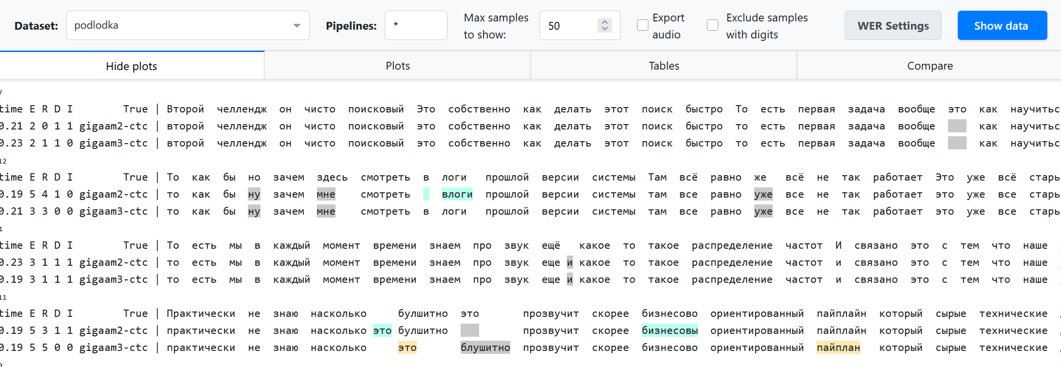
We use specific colors in 2 pipelines comparison mode, otherwise we just highlight errors in red.

Multi-environment mode¶

Many ASR models may have incompatible dependencies. To handle this, you may run asr_eval.bench.run from specific environments with model installations, and then run asr_eval.bench.dashboard.run from another environment. See:doc:guide_installation for installation instructions.

Dataset specs¶

We provide extended CLI syntax to specify custom audio processing, text processing and sample count. Instead of a dataset name, you can provide a semicolon-separated string, where the first value is a name pattern, other values are modifiers in form <key>=<value> (see also DatasetSpec).

We will provide the examples below.

Dataset modifiers¶
Modifier	Meaning
`a={name}`	Use custom audio preprocessor with `{name}`.
`p={name}`	Use custom tokenizer/normalizer with `{name}`.
`n={number}`	Run only the first `{number}` samples from the datset.
`n={number}!`	The `!` mark has no effect when running pipelines, and when running dashboard it will compare pipelines on exactly this count of samples. This will skip loading all subsequent samples, and samples skip all pipelines that don’t have predictions for full set of these samples.
`n=all!`	Same as previous, but all is treated as “all samples for this dataset”. I. e. this will skip loading pipelines that have only partial predictions.

Limiting sample count¶

Imagine that we define 2 benchmarks:

Our full benchmark contains a full podlodka dataset and the first 20 samples of the fleurs-ru dataset.
Our tiny benchmark (for quick validations) contains the first 5 samples of podlodka and fleurs-ru.

We will run gigaam2-ctc and gigaam2-rnnt-vad in full benchmark, and whisper-tiny on tiny benchmark.

FULL_BENCH="podlodka:n=all! fleurs-ru:n=20!"
TINY_BENCH="podlodka:n=5! fleurs-ru:n=5!"
GIGA="gigaam2-ctc gigaam2-rnnt-vad"
WHISPER="whisper-tiny"
python -m asr_eval.bench.run -d $FULL_BENCH -p $GIGA -s predictions
python -m asr_eval.bench.run -d $TINY_BENCH -p $GIGA $WHISPER -s predictions

The second command will skip running GigaAM pipelines, because the predictions were already saved: full benchmark includes all samples from tiny benchmark.

Now we can run the dashboard for full benchmark:

python -m asr_eval.bench.dashboard.run -d $FULL_BENCH -s predictions -c dashboard_cache

Note that whisper-tiny is not shown in the dashboard, since it does not have predictions for full benchmark. If we had removed :n=all! and :n=20! from the benchmark definition, the dashboard would have loaded whisper-tiny also, and since it has only 5 predictions per dataset, metrics in “plot” section would have been averaged over 5 samples, that is undesired.

We can also run the dashboard for tiny benchmark:

python -m asr_eval.bench.dashboard.run -d $TINY_BENCH -s predictions -c dashboard_cache

Now only 5 samples are loaded for all pipelines. This ensures that we compare pipelines on the data we intended to use.

Example benchmark¶

We provide an example bench.sh of what a real production-level ASR benchmark looks like. We removed some datasets and anonymized internal models.

The file contains several dataset bundles, and run each model type in its own environment. For example, the DATASETS_CHECK bundle is made to quickly decect possible regression in new versions of internal models or their embedded versions, where running on the full benchmark would be an overhead.

Adding custom dataset¶

Let’s create a Python module my_module.py and register a new dataset of Spanish femals speech. We need to write a dataset loading function and decorate it with @register_dataset, using a unique name.

Dataset should contain the following fields per sample:

“audio” - a float32 waveform with sampling rate 16000, usually normalized roughly from -1 to 1.
“transcription” - the ground truth transcription, possibly multivariant or not.
“sample_id” - a unique (within the current dataset and split) sample index.

from datasets import Audio, load_dataset, Dataset
from asr_eval.bench.datasets import register_dataset
from asr_eval.bench.datasets.mappers import assign_sample_ids

@register_dataset('spanish')
def load_spanish(split: str = 'test') -> Dataset:
    return (
        load_dataset(
            'ylacombe/google-chilean-spanish',
            name='female',
            # asr_eval uses "test" split in asr_eval.bench.run
            # however, when a single split is provided, HF calls it "train"
            # due to this limitation, we need to refer to it as "test"
            split='train',
        )
        # asr_eval requires "transcription" column
        .rename_column('text', 'transcription')
        .cast_column('audio', Audio(sampling_rate=16_000))
        # asr_eval requires "sample_id" column
        # to track samples identity after shuffling the dataset
        .map(assign_sample_ids, with_indices=True)
    )

See examples in the asr_eval.bench.datasets._registered package. See Datasets usage. for more information about programmatic usage of datasets in asr_eval and sample enumeration.

Now we can run whisper-tiny and look at the results. To import out new module, we use --import my_module argument.

python -m asr_eval.bench.run -p whisper-tiny -d spanish:n=10 \
    --import my_module -s predictions
python -m asr_eval.bench.dashboard.run -d spanish \
    --import my_module -s predictions -c dashboard_cache

Adding custom pipeline¶

Let’s find some spanish models on HuggingFace and build a composite pipeline. We use a LongformCTC that wraps a CTC model, performs inference on uniform chunks and merge them. However, because our Spanish dataset contain short audios, this will have no effect and we could drom this wrapper.

from huggingface_hub import hf_hub_download # type: ignore

from asr_eval.bench.pipelines import TranscriberPipeline
from asr_eval.ctc.lm import CTCDecoderWithLM
from asr_eval.models.base.longform import LongformCTC
from asr_eval.models.wav2vec2_wrapper import Wav2vec2Wrapper


class _(TranscriberPipeline, register_as='spanish-wav2vec-lm'):
    def init(self):
        return CTCDecoderWithLM(
            LongformCTC(
                Wav2vec2Wrapper('LuisG07/wav2vec2-large-xlsr-53-spanish')
            ),
            hf_hub_download('kensho/5gram-spanish-kenLM', 'kenLM.arpa'),
        )

See examples in the asr_eval.bench.pipelines._registered package.

Since we KenLM here, run bash installation/kenlm.sh from the asr_eval repo to install the required additional dependencies. then we can run the model and view the results.

python -m asr_eval.bench.run -p spanish-wav2vec-lm -d spanish:n=10 \
    --import my_module -s predictions
python -m asr_eval.bench.dashboard.run -d spanish \
    --import my_module -s predictions -c dashboard_cache

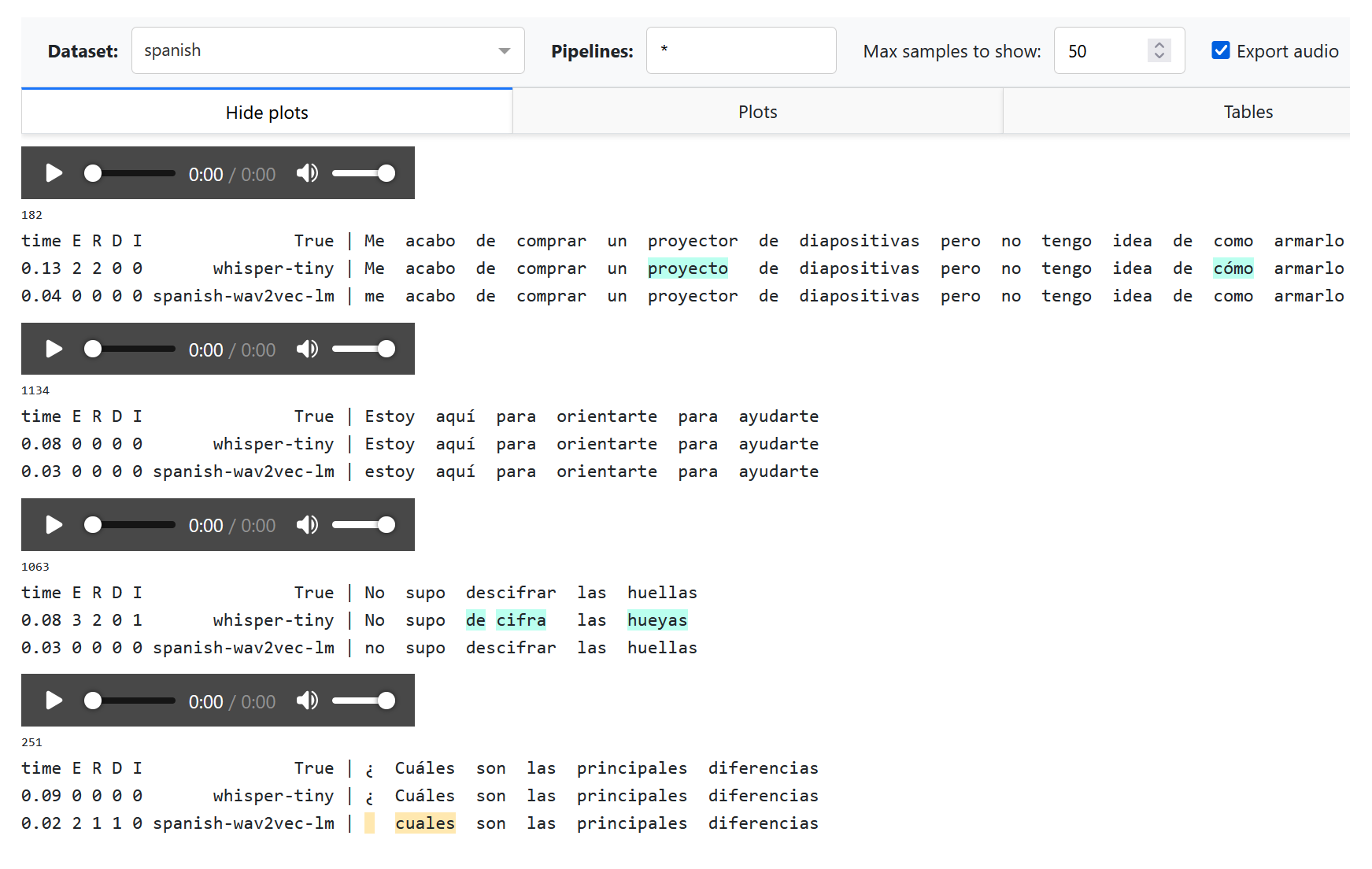
Note that the “¿” is treated as missing word becuse is not recognized as a standard punctuation symbol. We can handle this with a custom text processor.

Pipelines are not parametrized. Parametrization would introduce many complexities with 1) tracking if the results are already calculated or not, 2) specifying the same parameters to reproduce the results, 3) adding hyperparameters that were previously hardcoded. Thus if you want to try multiple hyperparameter values, you need to create multiple pipelines.

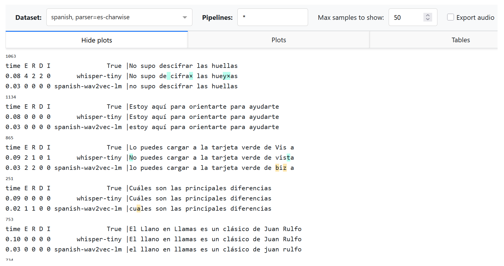
Adding custom tokenizer or preprocessor¶

Let us want to switch to character-based alignment, treating any character or space as a word, but ignore punctuation symbols, including the “¿” symbol. To this end, we need to modify a word regexp in a parser (see the default regexp here). We also add a custom preprocessing function to remove the leading space generated by Whisper.

from asr_eval.align.parsing import PUNCT, Parser
from asr_eval.bench.parsers import register_parsers

class CharWiseParser(Parser):
    def __init__(self):
        super().__init__(
            tokenizing=rf'[^{PUNCT}¿]',
            preprocessing=lambda text: text.lstrip(),
        )

register_parsers(
    'es-charwise',
    # register the same parser for both annotation...
    true_parser=CharWiseParser,
    # ...and prediction
    pred_parser=CharWiseParser,
)

Now we can test our modifications on the previous predictions:

ASR_EVAL_CHARWISE_RENDER=1 python -m asr_eval.bench.dashboard.run \
    -d spanish:p=default,es-charwise \
    --import my_module -s predictions -c dashboard_cache

Explanations:

We still add --import my_module, where now we have a new dataset, new pipeline and a new parser (i. e. tokenizer and preprocessor).
We use a comma-separated list of parsers p=default,es-charwise to try both default and new parser. Thus, we now see two datasets in the dropdown list: “spanish” and “spanish, parser=es-charwise”.
With ASR_EVAL_CHARWISE_RENDER=1, additional whitespaces will not be added on HTML rendering stage, and deletions will be marked as “×” symbol. Note that the default (word-based) parser will now be rendered incorrectly due to this option.
Changing parsers does not require re-generating predictions. Alignments for all parsers will be cached in a directory provided as -c argument, and will not interfere with each other.

Adding custom noise overlay¶

Let us apply an effect of bad microphone by cutting frequencies lower than 700-800 Hz and higher than 1500-1800 Hz. To do this, we again append the code to my_module.py.

We will use a library that can be installed with pip install audiomentations.

from asr_eval.bench.augmentors import AudioAugmentor
from asr_eval.bench.datasets import AudioSample

class _(AudioAugmentor, register_as='mic-noise'):
    def __init__(self):
        from audiomentations import Compose, LowPassFilter, HighPassFilter
        self.transform = Compose([
            LowPassFilter(1500, 1800, p=1.0),
            HighPassFilter(700, 800, p=1.0),
        ])

    def __call__(self, sample: AudioSample) -> AudioSample:
        sample = sample.copy()
        sample['audio']['array'] = self.transform(
            sample['audio']['array'],
            sample_rate=sample['audio']['sampling_rate'],
        )
        return sample

You can define a meaningful class name, but this is not required, because the object will be retrived by a component name. We can test this:

import my_module  # where we defined "mic-noise" processor
from IPython.display import display, Audio
from asr_eval.bench.augmentors._registry import get_augmentor
from asr_eval.bench.datasets import get_dataset

augmentor = get_augmentor('mic-noise')
sample = get_dataset('podlodka')[0]
display(Audio(sample['audio']['array'], rate=16000))  # before
sample = augmentor(sample)
display(Audio(sample['audio']['array'], rate=16000))  # after

Conceptually, AudioAugmentor defines a fixed preset used for model inference. It represents a chain of operations with concrete parameters. However, it should not necessarily be deterministic. Only a single AudioAugmentor can be used during inference: if you need to combine many, then write another AudioAugmentor that combines these operations, and register under a new unique name.

We can now perform inference with our new augmentor. We will use a Fleurs Ru subset and Whisper-tiny model.

python -m asr_eval.bench.run -p whisper-tiny \
    -d fleurs-ru:n=50 fleurs-ru:n=50:a=mic-noise \
    --import my_module -s predictions
# importing audio ops is not required when running a dashboard
python -m asr_eval.bench.dashboard.run -d fleurs-ru:n=50 \
    -s predictions -c dashboard_cache

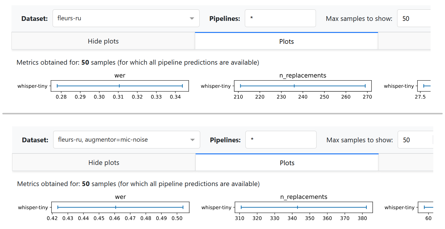
As expected, the deterioration of the sound increased the number of errors. Note that currently the dashboard does not show audio with noise overlays on “Export audio”.

Streaming diagrams¶

TODO.

Datasets usage¶

You can get a registered dataset via get_dataset() function:

from asr_eval.bench.datasets import AudioSample, get_dataset

dataset = get_dataset('podlodka')
sample: AudioSample = dataset[0]

A default split is “test”, which is also used in asr_eval.bench.run for inference, but some datasets may provide other splits (train, validation):

dataset = get_dataset('podlodka', split='train')

Note that we indentified and removed duplicates in several datasets to prevent train-test leakage. If we found the same audio (up to maybe a different magnitude ans slicing) in train and test, we remove if from test. If we found the same audio twice or more in a single split, we also remove these duplicates. Technically, we store sample IDs for duplicates and remove them on the fly when loading a dataset. To disable this, pass filter=False:

dataset = get_dataset('podlodka', filter=False)

Datasets are shuffled with seed 0 by default. With shuffling, the first N samples form a representative set of the whole dataset (often Hugging Face datasets are not shuffled in advance). When you shuffle a dataset, “sample_id” field helps to track the sample identity. That’s why when you run asr_eval.bench.run -d {dataset}:n=10, the processed samples seem to have “random” ids and not from 0 to 9. Actually, these are the first 10 samples in the shuffled version. To disable shuffling, pass shuffle=False (asr_eval.bench.run does not suport this for now):

dataset = get_dataset('podlodka', shuffle=False)

Note that in get_dataset shuffling happens before filtering and therefore shuffled sample order does not alter when you toggle filter parameter.

To list all available datasets and splits, see the Datasets list page or run:

from asr_eval.bench.datasets import datasets_registry

for dataset_name, dataset_info in datasets_registry.items():
    print('dataset:', dataset_name, 'splits:', dataset_info.splits)